A carrier uses 30 kHz subcarrier spacing. Does that mean it is faster than a 15 kHz carrier?
No. It means the time-frequency grid is organised differently.
Subcarrier spacing affects symbol and slot structure. It does not tell you how many PRBs a UE received, which MCS was selected, how many layers were realised, how much retransmission occurred, whether the TDD pattern offered a downlink opportunity, or whether the test path was limited beyond the RAN.
The field sequence is:
- establish the configured grid;
- verify that the band, channel bandwidth and SCS combination is supported;
- identify the carrier and BWP context actually used;
- separate the design objective from the observed symptom;
- test other explanations before recommending a numerology change.
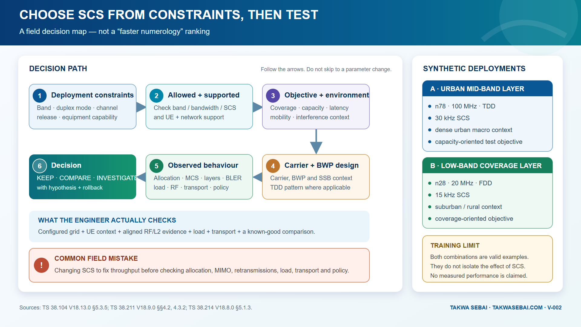
Original Takwa Sebai decision map. The two deployment examples are synthetic and are not an A/B performance comparison.
The basic NR numerology relationship
For NR:
Δf = 2^μ × 15 kHz
where μ is the numerology index.
For the normal cyclic-prefix examples used here:
| μ | Subcarrier spacing | Slots in 1 ms | Reference slot duration | OFDM symbols per slot |
|---|---|---|---|---|
| 0 | 15 kHz | 1 | 1 ms | 14 |
| 1 | 30 kHz | 2 | 0.5 ms | 14 |
| 2 | 60 kHz | 4 | 0.25 ms | 14 |
| 3 | 120 kHz | 8 | 0.125 ms | 14 |
The reference slot duration is the 1 ms subframe divided by the number of slots in that subframe. It is useful for reading the grid. It is not an end-to-end latency promise.
As μ increases:
- the SCS doubles;
- the useful OFDM symbol period becomes shorter;
- the number of slots in the same 1 ms interval doubles;
- the grid can represent scheduling opportunities at a finer time granularity.
The word can is essential. A shorter slot does not prove the scheduler served a UE sooner or the packet crossed the entire service path faster.
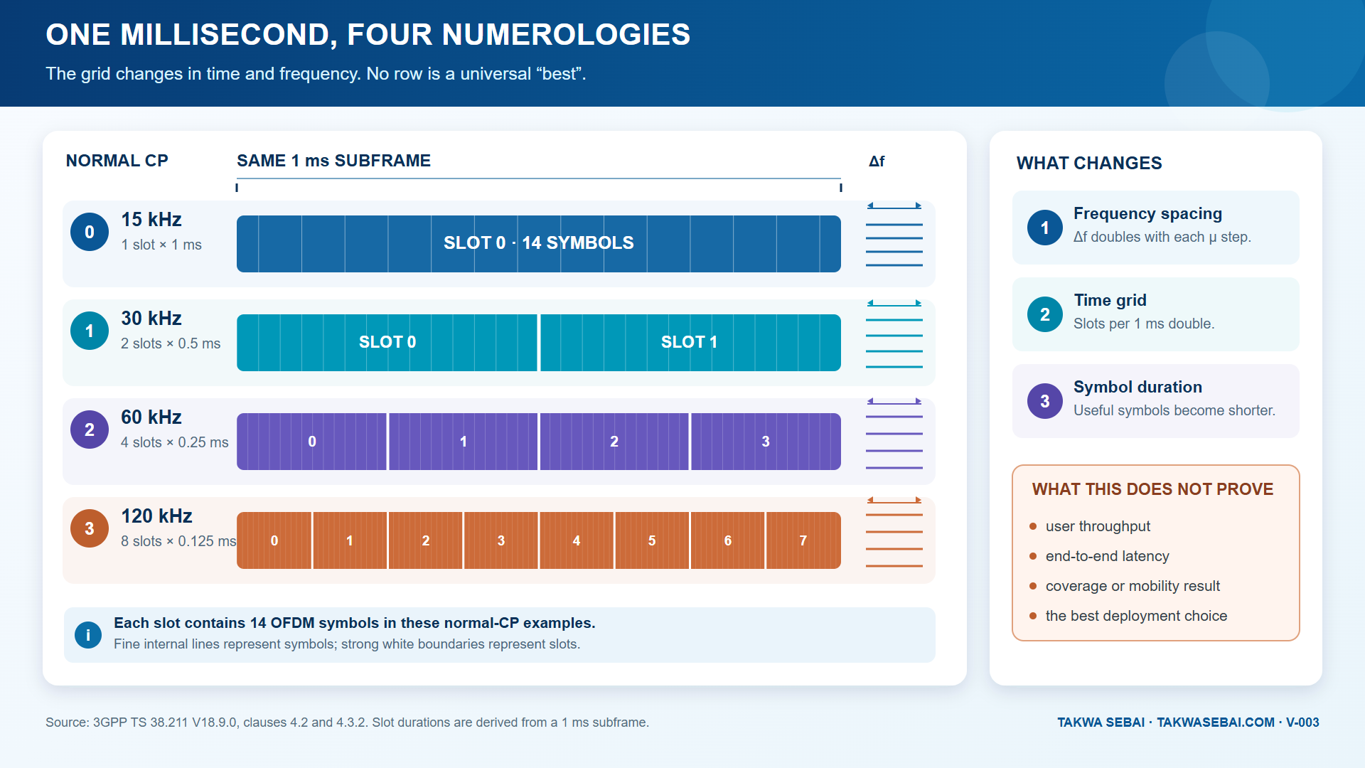
Original Takwa Sebai time-frequency comparison. More slot boundaries do not mean more user throughput by themselves.
Read the time and frequency axes together
Time view
Inside the same 1 ms subframe:
- 15 kHz SCS has one reference slot;
- 30 kHz has two;
- 60 kHz has four;
- 120 kHz has eight.
This does not show which symbols are downlink, uplink or flexible in a TDD configuration. It also does not show whether the scheduler assigned resources to the UE.
Frequency view
A larger SCS places adjacent subcarriers farther apart. The resource grid therefore changes in frequency as well as time.
The deployed design also has a band, channel bandwidth, BWP context, SSB configuration, duplex mode, antenna system and real propagation environment. “Shorter slot” describes only one part of that design.
What the grid does not contain
A numerology diagram does not tell you:
- allocated PRBs;
- modulation order or target code rate;
- realised MIMO layers;
- BLER, HARQ or other retransmission pressure;
- cell load and scheduler decisions;
- TDD direction opportunities;
- protocol overhead;
- transport and core limitations;
- subscription, server or device limits.
Treat the grid as a coordinate system, not a performance result.
Check constraints before preferences
The first engineering question is not “Which SCS is best?” It is “Which combinations are defined and supported for this deployment?”
At minimum, establish:
- operating band and frequency range;
- duplex mode;
- configured channel bandwidth;
- carrier SCS and the SCS of the relevant BWP;
- SSB and common-configuration context;
- UE and network capability;
- software and feature baseline.
The applicable 3GPP release and product documentation still matter. A training article is not a substitute for the deployed equipment baseline.
This order also prevents false comparisons. A low-band FDD coverage layer and a mid-band TDD capacity layer differ in far more than numerology.
Why SCS is not a throughput button
Downlink transport-block determination depends on inputs including:
- modulation order;
- target code rate;
- number of layers;
- number of allocated PRBs.
This supports a narrow conclusion:
SCS alone is insufficient to determine user throughput.
It does not make SCS irrelevant. It means a throughput diagnosis must include the variables that determine how much data was scheduled and delivered successfully.
For a low-throughput investigation, align:
- serving carrier and active BWP;
- UE capability and serving mode;
- allocation across the test interval;
- modulation, coding, rank/layers and retransmission evidence;
- RF condition and mobility state;
- cell load and a comparison interval;
- TDD pattern where applicable;
- transport, server and test method;
- policy or subscription limits.
Only after this should numerology remain on the list of plausible limiting design factors.
Break the false causal chain
A common shortcut is:
30 kHz SCS → shorter slot → lower latency → higher throughput
Each arrow requires evidence.
- Shorter reference slot: a property of the grid.
- Lower radio delay: depends on the configured opportunity and actual scheduling.
- Lower end-to-end latency: depends on RAN, transport, core and application.
- Higher throughput: depends on resources delivered successfully over time.
The chain may guide a design discussion. It is not a field diagnosis.
Synthetic comparison: two deployment roles
These two scenarios are synthetic. They are not measured networks, customer cases or proof of the author's deployment practice.
| Attribute | Scenario A: urban mid-band | Scenario B: low-band layer |
|---|---|---|
| Band | n78 | n28 |
| Channel bandwidth | 100 MHz | 20 MHz |
| Duplex | TDD | FDD |
| SCS | 30 kHz | 15 kHz |
| Generic context | dense urban macro | suburban or rural |
| Training objective | capacity-oriented test | coverage-oriented test |
The cited Release 18 version of TS 38.104 supports these band, channel-bandwidth and SCS combinations.
What the comparison teaches:
- layers may have different network objectives;
- bandwidth and duplex opportunities must be considered;
- UE population and services matter;
- the evidence should be tied to the objective.
What it does not prove:
- that 30 kHz always means speed;
- that 15 kHz always means coverage;
- that SCS caused any performance difference;
- that one scenario has better latency or spectral efficiency;
- that the result would persist with different load, site grid, antenna or TDD pattern.
Those claims require controlled evidence.
Verify the deployed reality in three layers
Layer 1: planned and configured design
Preserve an authorised export or screenshot containing:
- band and duplex mode;
- channel bandwidth;
- carrier and BWP SCS;
- SSB/common configuration;
- TDD pattern where applicable;
- release, software and feature baseline.
Keep the object identity and timestamp. Do not rewrite the configuration from memory.
Layer 2: UE and signalling context
Use an authorised trace or device log to determine:
- the serving cell and carrier;
- NSA or SA context;
- the relevant BWP;
- reconfiguration during the test;
- mobility, fallback or another state transition.
Do not infer the active context from one isolated decoded field.
Layer 3: observed behaviour
Align:
- exact test start and stop time;
- location and radio conditions;
- UE model, capability and thermal state;
- allocation and load;
- retransmission and MIMO evidence;
- transport and server measurements;
- a known-good comparison.
Configuration describes intent. Traces and measurements describe what happened to this UE in this interval.
Decision workflows by symptom
Throughput below expectation
- Prove the test is repeatable.
- Confirm cell, carrier, mode and BWP.
- Verify band, bandwidth and SCS against the design.
- Inspect allocation, MCS, layers and retransmissions.
- Check load and TDD opportunities.
- Exclude transport, server, policy and UE limits.
- Compare with a known-good case using the same carrier design.
- Consider a controlled numerology trial only if the evidence still points there.
Latency above expectation
Separate:
- scheduling and retransmission delay;
- TDD waiting time;
- RAN processing and queues;
- transport and core;
- server and application response;
- measurement resolution and clock alignment.
A 0.5 ms reference slot cannot explain a 30 ms end-to-end result on its own.
Coverage or mobility unstable
Verify:
- band and antenna/beam context;
- serving and neighbour measurements;
- SSB and measurement configuration;
- handover or beam-management phase;
- speed and route repeatability;
- timing, interference and retransmission evidence.
Numerology is not a substitute label for every RF trade-off.
Before changing SCS
Reject a proposal such as “speed is low, use a wider SCS” until it defines:
- why the current combination is wrong or limiting;
- whether allocation, MIMO and delivery are healthy;
- whether transport and policy are excluded;
- whether the alternative is supported;
- what observation would confirm success;
- what would falsify the hypothesis;
- the service risk and rollback;
- the comparison window and acceptance criterion.
A change should answer a measured question. It should not be an experiment performed because the grid diagram looks faster.
Minimum evidence package
| Area | Required evidence |
|---|---|
| Configuration | release, band, duplex, bandwidth, carrier/BWP SCS, SSB/TDD context |
| Test | cell, interval, UE, mode, route, server, duration and load |
| Radio delivery | allocation, MCS, rank/layers, BLER/HARQ and TDD opportunity |
| End-to-end | transport, server and policy checks |
| Decision | hypothesis, alternative causes, falsifier, rollback and real baseline |
Continue the evidence chain
- Prove which BWP was active.
- Read RSRP, RSRQ and SINR together.
- Use the complete low-throughput workflow.
- Read the complete 5G NR field guide.
Download the free illustrated 111-page ebook.
Technical sources
- 3GPP TS 38.211 V18.9.0, Release 18, clauses 4.2 and 4.3.2 for SCS and normal-CP slot structure. ETSI publication.
- 3GPP TS 38.104 V18.13.0, Release 18, clause 5.3.5 for channel-bandwidth/SCS combinations. ETSI publication.
- 3GPP TS 38.214 V18.8.0, Release 18, clause 5.1.3 for transport-block determination inputs. ETSI publication.
KEEP THE EVIDENCE PATH